Excel Tips
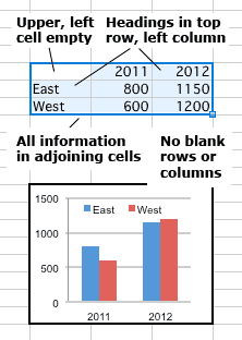
from selected data.
Excel makes it easy to plot data in charts provided the information is set up correctly. The following guidelines work for most chart types:
- Enter all the headings and chart data in one block.
- Place headings on the top-most row and left-most column.
- Leave the upper, left corner cell empty. That helps Excel identity the headings.
- Do not leave blank rows and columns within the area to be plotted unless you eventually intend to fill them with data.
TRADITIONAL DIALOGUE BOXES IN EXCEL 2007 AND 2010.
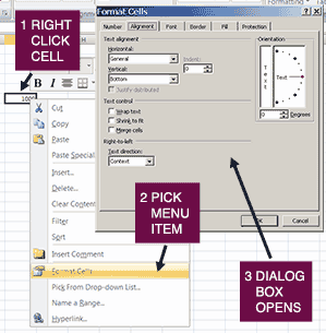
dialogue boxes for many features.
If you miss the familiar menus and dialogue boxes of Excel 2003, you can access many of them by right-clicking. For example, to get the traditional Format Cells dialogue box --
- Select the cells you want to format.
- Right click on the selected area.
- Choose the desired command from the menu.
COMBINING TEXT: AMPERSAND OR CONCATENATE FUNCTION.
Many people use the Concatenate function to combine several text strings into one. For example, the formula
=CONCATENATE("Boston",", ","Massachusetts")
produces the result
Boston, Massachusetts
Often, however, it is easier to use the text operator, "&" to achieve the same result. The formula would be
="Boston" & ", " & "Massachusetts"
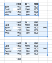
To select an entire block of data --
- Click on any non-blank cell within the region you want to select. That is now the "Active Cell."
- Press Control+A (Windows) or Command+A (Macintosh).
The selection continues up, down, left and right from the Active Cell until it can go no further without jumping an empty cell.
DRAG-AND-DROP COPYING.
Excel’s drag-and-drop editing feature lets you move the contents of one or more cells by selecting the cells to be moved, placing the tip of the mouse pointer anywhere on the border of the selection except the AutoFill handle in the lower right corner, and dragging the selection to its destination. To copy the selection instead of moving it, press the Control (Windows) or Command (Macintosh) key while dragging.
PRINTING PORTION OF WORKSHEET.
There are two ways to tell Excel to print a specified area of a worksheet --
- To print a portion of a worksheet on a one-time basis, select the cells to be printed. Then in the "Print" dialogue box, choose "Selection" from the "Print What" options.
- To save the designation of the print area with the spreadsheet, open the "Page Setup" dialogue box ("File" menu) and click the "Sheet" tab. Enter the cell range to be printed in the "Print Area" box.
CREATING A CUSTOM AUTOFILL SERIES.
Excel has certain commonly-used series programmed into its AutoFill feature, days of the week for example.
But you can also create a custom series by providing a sample. Here is how --
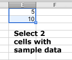
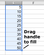
- Enter the first two series values in adjoining cells. For example, to create a series of integers 5, 10, 15, 20 …, enter 5 and 10.
- Select (highlight) the two sample cells.
- Place the mouse on the "fill handle" in the lower right corner of the selected area.
- Drag the mouse across the cells into which you want the series to be entered. In our example those cells would be filled with 15, 20, 25, etc.
AVOIDING GAPS IN CHARTS.
A common problem in creating Excel charts is how to eliminate gaps created by rows and columns in the data worksheet that intentionally have been left empty. Excel treats them as having a value of zero and plots them accordingly.
In many cases you can avoid this problem by entering the data without the empty cells, creating the chart, and then inserting the empty rows or columns. Excel will automatically maintain the linkages between the chart and the correct data cells in the worksheet.
This technique will not work where the insertion adds a category. In those cases you will have to tell the ChartWizard exactly which cells to plot. To do so, go to Step 1 in the ChartWizard and delete the entries in the "Range" box. Then highlight the cells containing the data you wish to plot. To skip empty cells, press the Control (Windows) or Command (Macintosh) key while highlighting the cells you want to include. Be sure to highlight the row and column titles in the worksheet if you want them added to the chart. Then proceed as usual with the remaining steps in creating the chart.
ADJUSTING COLUMN WIDTH TO FIT CONTENTS.
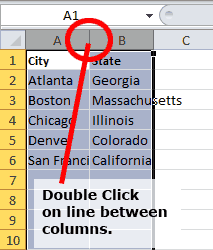
To adjust the width of one or more columns to fit the largest cell entry in each --
- Select the columns to be adjusted;
- Place the mouse pointer on the divider between any two column headings within the selected area (the heading is the gray box with a letter inside at the top of each column); and
- Double click the mouse button.
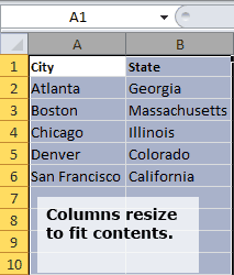
Each selected column will enlarge or shrink so that it exactly fits the longest entry under it.
To link Excel workbooks easily, let Excel make the necessary entries for you. Here’s how:
- Make sure the source and linked worksheets are saved where you intend to keep them since the linkage records the exact locations of the files.
- Open both worksheets, placing them side by side. The Arrange command (Window menu) can do this for you.
- If necessary, scroll through the worksheets until the cells to be linked are both visible
- Begin the formula in the linked cell.
- Click twice on the source cell. The first click activates the source worksheet, the second enters the cell reference.
- Complete your formula; press Enter.
Excel Training Class · Excel Tech Support

